OEIS/FASS curves
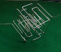
Beyond OEIS sequence A220952
After my initial attemps to extend sequence A220952 I became interested in FASS curves in general.
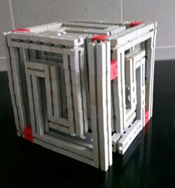
Sequence A220952 is best discussed with numbers to base 5. The first 125 values then are:
0,
1,2,3,4,
14,24,34,33,32,31,21,22,23,13,12,11,10,20,30,40,41,42,43,44,
144,244,344,343,342,341,241,242,243,143,142,141,140,240,340,
330,320,310,210,220,230,130,120,110,111,112,113,123,122,121,
131,132,133,233,232,231,221,222,223,213,212,211,311,312,313,
323,322,321,331,332,333,334,324,314,214,224,234,134,124,114,
104,204,304,303,302,301,201,202,203,103,102,101,100,200,300,
400,401,402,403,404,414,424,434,433,432,431,421,422,423,413,
412,411,410,420,430,440,441,442,443,444
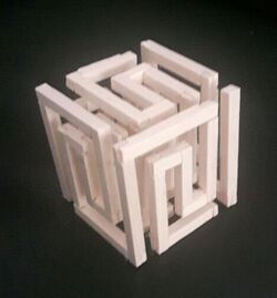
In each generation the number of digits is increased by one. The first 25 values form the adjacency condition matrix as defined by Knuth:
       Kn
04==14==24==34  44
||          ||  ||
03  13==23  33  43
||  ||  ||  ||  ||
02  12  22  32  42
||  ||  ||  ||  ||
01  11  21==31  41
||  ||          ||
00  10==20==30==40
Here, the last digit is the y coordinate, and the digit before is the x coordinate. In generation 3, the left-most digit can be interpreted as the z coordinate. Since this is Knuth's original adjacency matrix, and since it shows a path similiar to a letter n inside the square, I named it "Kn".
The curve is space-filling in every dimension
For the cube I wrote a Javascript program with the beautiful framework three.js.
A Go package for Hilbert and Peano curves can be found on github.com.
Variants
Next I wrote a Perl program which always starts with nodes 00, 01, but which then exhausts all possible paths which fill the 5*5 square. That program found several adjacency matrices which have similiar properties like that of Knuth. Depending the shapes of the paths, I invented names for them:
        Fs                    Ls                    Ln                    NN
04==14==24==34  44    04==14  24==34==44    04==14  24==34  44    04==14  24==34  44
||          ||  ||    ||  ||  ||            ||  ||  ||  ||  ||    ||  ||  ||  ||  ||
03  13==23==33  43    03  13  23==33==43    03  13  23  33  43    03  13  23  33  43
||  ||          ||    ||  ||          ||    ||  ||  ||  ||  ||    ||  ||  ||  ||  ||
02  12==22==32  42    02  12  22==32==42    02  12  22  32==42    02  12  22  32  42
||          ||  ||    ||  ||  ||            ||  ||  ||            ||  ||  ||  ||  ||
01  11==21==31  41    01  11  21==31==41    01  11  21==31==41    01  11  21  31  41
||  ||          ||    ||  ||          ||    ||  ||          ||    ||  ||  ||  ||  ||
00  10==20==30==40    00  10==20==30==40    00  10==20==30==40    00  10==20  30==40
For these 4 matrices I checked the uniqueness of the generated paths up to n=3125 (5th dimension). Proofs similiar to that for sequence A220952 can probably be devised for these matrices, too.
You may look at:
- "Fs" as a colored line with coordinates
- "Fs" as a solid 3D model
- more examples, also for bases 2..7
Different Bases
Searching for space filling paths reminds me a bit to the famous OEIS stamp folding sequence A001011. The Perl program mentioned above finds following numbers of space filling matrices for bases 1, 2, 3 ...;
base count examples and notes
1      1   (a single node)

2      1   01==11  first order Hilbert curve
           ||  ||
           00  10
                                                         n
3      4   02==12==22    02==12==22    02==12==22    02==12  22
                   ||    ||      ||    ||      ||    ||  ||  ||
           01==11  21    01  11==21    01  11  21    01  11  21
           ||  ||  ||    ||  ||        ||  ||  ||    ||  ||  ||
           00  10==20    00  10==20    00  10==20    00  10==20
4     26
5    412   where 5 generate paths up to the 5th dimension
6  11072
...    ?
The basic building block (for odd bases) seems to be the last matrix for base 3 above. Only this one generates a path (up to the 6th dimension).
Examples
| Base | Variants |
| 2 | u |
| 3 | N - simple wave, nucleus of Kn |
| 4 | M - probably not extensible to 4th dimension |
| 5 | Kn - Knuth's original OEIS sequence A220952 Fs - center turned Ln - asymmetric, similiar to Kn Ls - asymmetric, similiar to Fs NN - simple wave |
| 6 | W - probably not extensible to 4th dimension |
| 7 | Kn7 - like Kn, c.f. A300857 IssI, another shape LnT, yet another |
| 9 | some example (id="34862") |
For your own experiments, you may use the DIY meander cube page. You may specify whether labels should be attached, in decimal or in the "natural" base, and you can even export an STL file there.
3D Manufacturing
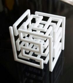
All my attempts to physically build such objects were unsatisfying so far. The balsa lumber and the Fischertechnik (above) approaches worked somehow, but both needed distance bars (thin needles for the balsa, red blocks for Fischertechnik) to keep the geometry in shape. Cutting and glueing the 62 balsa parts was very tedious.
In discussions with several people I learned that such FASS curves cannot be produced by conventional processes like milling or die casting. Therefore I tried the current hype of 3D printing.
With Three.js it is also very easy to store an STL file derived from the virtual scene. STL is the main format for stereolithography CAD software, 3D printers and other manufacturing devices. STL stores a mesh, that is a set of triangles representing the geometry of the object.
- Download the meander STL file and view it with the free service of viewstl.com, and/or
- send the STL file to the production service company of your choice.
During my holidays in Greece I sent this a file to trinckle.com in Germany, and within 10 days and 20 € I received the nice 4x4 cm cube on the right. It was made by sintering plastic (polyamide) with a laser. The problem is that the structure cannot be built on a supporting surface, and that there is some warping caused by the heat of the laser and the weight of the material. The object is very fragile.
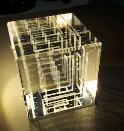
In the next step I ordered a 5x5x5 cm bubblegram, an internally engraved glass cube from easycrystal.de for about 40 €. Such a cube is very stable, and the engraved point cloud for the FASS curve is geometrically exact. In addition to the curve the base 5 coordinates are shown, but they are very tiny. The STL file should probably be "cleaned" from triangles inside the bars. There is a good overview of 7 free STL editors, among them MeshMixer.
Observations and efficiency considerations
A brute-force, backtracking algorithm which generates all pathes for a specific base runs rather fast up to base 5 (412 possible paths). For base 7, there are about 3 millions of paths starting with 00~01 ("~" denotes "adjacent to"), but only 47 of them can be continued in dimensions > 2. For base 9, the brute-force approach is not feasible, and it is necessary to develop restrictions for the backtracking algorithm.
For the following discussion, let digits b = base-1, a = b-1, c=b+1, h=a/2, and for elements (n, n) on the diagonal, m=n-1, p=n+1. For a node, we will write xy instead of (x,y), and zxy instead of (z,x,y). hh is the center element, {00, 0b, bb, b0} is the set of corner elements. Let st be the coordinates of the start point, and ef those of the end point.
0b  1b  ..  ab  bb      ..  ..  ..  ..  ..

0a  1a  ..  aa  ba      ..  mp  np  pp  ..

..  ..  hh  ..  ..      ..  mn  nn  pn  ..

01  11  ..  a1  b1      ..  mm  nm  pm  ..

00  10  ..  a0  b0      ..  ..  ..  ..  ..
The path must visit every node in the square of the adjacency matrix exactly once, and so it must in the d-dimensional cubes (for d >= 3) of edge length base. Furthermore, any projection of such a cube to the plane must show the same adjacency matrix (for odd bases; even bases are discussed later). In essence, any projection must not show some "T" pattern:
mn==nn==pn        mp
    ||            ||
    nm      or    mn==nn
                  ||
                  mm
Start and end points in some corner
The start point starts the multidimensional path, and the end point is the last path element in the square, 2-dimensional adjacency matrix. At the end point, the path continues into the 3rd dimension (z=1), It is natural to assume a start point 00, and experiments show that the end point then always is the opposite corner bb for continuing paths. BTW, there are continuing paths which are not rotational symmetric (e.g. Ls and Ln for base 5).
- The start and the end point both are corner elements.
Otherwise, they will show a "T" pattern in one of the projections zx, zy.
Normalization 00~01
- We may always start with 00~01 without loss of generality.
There are 7 equivalent paths starting with 00~10, 0b~0a, 0b~1b, bb~ab, bb~ba, b0~1b, b0~a0. Therefore only one set needs to be computed.
Diagonal start and end point
- Start and end point are in opposite corners.
With the normalized start 00~01, and 0b as end point, we get 00b~10b, and therefore 00~10, a contradiction. With b0 as end point, we get 0b0~1b0, and the same contradiction 00~10. Therefore, the end point must be bb.
Straight left edge
- The path starts with 00, 01, 02, ...0b.
If there is any deviation 0n~1n with 0 < n < b, then the corresponding diagonal element 0nn has, in addition to its 2 normal neigbours in the adjacency matrix, a 3rd neighbour 1nn in the next z plane.
The path may not divide the square
- If the path hits a border, one of the 2 neighbouring nodes must already be contained in the path.
If both neighbours were not visited so far, the path would divide the square in 2 halves, It would turn into one of them, and could never reach the non-visited nodes in the other one.
Elementary waves on the diagonal
It appears that continuing paths must contain wave shapes at least on one of the diagonal nodes 22, 33 .. aa. The 3-wave has the "n" shape, the 5-wave looks like "NN", and in general the b-wave is 00~01..0b~1b~1a..10~20..2b..ba~bb. The shapes on the diagonal nodes will be rotated, but only in 2 out of 4 possible ways, depending on the parity of the row number.
No "stairs"
It seems - at least for odd bases - that path segments which change the direction 4 times (or more often) in a row are not allowed:
XX==XX            XX==XX
    ||                ||
    XX==XX   or   XX==XX
        ||        ||
        XX        XX
Implementation
The Perl program gen_paths.pl uses the restrictions mentioned above.
Path expressions
In order to prove the desired properties, we will use a language which describes the paths up to some generation (dimension). We use the following operations to build path expressions:
- A0 = [] : the empty path
- X = [a,b,c] : build a path expression X from elements a,b,c
- "/X" : reverse the sequence of elements in path expression X
- "X.n+m" : insert digit m after the digit for base^n in each element of X
Examples:
[].0+1 = [1];
[12].0+3 = [123];
[12].2+3 = [312];
[1234].1+0 = [12304];
With this notation, we can describe the paths for base 3 and base 5 in a rather consistent way. It should be obvious how additional expressions must be added for higher dimensions. Similiar shapes show very similiar path expressions.
Base 3
n      A0 = [];
       A1 = [A0.0+0,/A0.0+1,A0.0+2];
       A2 = [A1.1+0,/A1.1+1,A1.1+2];
       A3 = [A2.2+0,/A2.2+1,A2.2+2];
       ...
s      A0 = [];
       A1 = [A0.0+0,/A0.0+1,A0.0+2];
       A2 = [A1.0+0,/A1.0+1,A1.0+2];
       A3 = [A2.0+0,/A2.0+1,A2.0+2];
       ...
Base 5
Fs     A0 = [];
       A1 = [A0.0+3,/A0.0+2,A0.0+1];
       B1 = [A0.0+0,/A1,A0.0+4];
       A2 = [A1.0+3,/A1.0+2,A1.0+1];
       B2 = [A1.0+0,/A2,A1.0+4];
       C2 = [B1.1+0,/B2,B1.1+4];
       A3 = [A2.0+3,/A2.0+2,A2.0+1];
       B3 = [A2.0+0,/A3,A2.0+4];
       C3 = [B2.1+0,/B3,B2.1+4];
       D3 = [C2.2+0,/C3,C2.2+4];
       ...
Kn     A0 = [];
       A1 = [A0.0+3,/A0.0+2,A0.0+1];
       B1 = [A0.0+0,/A1,A0.0+4];
       A2 = [A1.1+3,/A1.1+2,A1.1+1];
       B2 = [A1.0+0,/A2,A1.0+4];
       C2 = [B1.1+0,/B2,B1.1+4]
       A3 = [A2.2+3,/A2.2+2,A2.2+1];
       B3 = [A2.0+0,/A3,A2.0+4];
       C3 = [B2.1+0,/B3,B2.1+4];
       D3 = [C2.2+0,/C3,C2.2+4];
       ...
Ln     A0 = [];
       A1 = [A0.0+2,/A0.0+3,A0.0+4];
       B1 = [A0.0+0,/A0.0+1,A1];
       A2 = [A1.1+2,/A1.1+3,A1.1+4];
       B2 = [A1.0+0,/A1.0+1,A2];
       C2 = [B1.1+0,/B1.1+1,B2];
       A3 = [A2.2+2,/A2.2+3,A2.2+4];
       B3 = [A2.0+0,/A2.0+1,A3];
       C3 = [B2.1+0,/B2.1+1,B3];
       D3 = [C2.2+0,/C2.2+1,C3];
       ...
Ls     A0 = [];
       A1 = [A0.0+2,/A0.0+3,A0.0+4];
       B1 = [A0.0+0,/A0.0+1,A1];
       A2 = [A1.0+2,/A1.0+3,A1.0+4];
       B2 = [A1.0+0,/A1.0+1,A2];
       C2 = [B1.1+0,/B1.1+1,B2];
       A3 = [A2.0+2,/A2.0+3,A2.0+4];
       B3 = [A2.0+0,/A2.0+1,A3];
       C3 = [B2.1+0,/B2.1+1,B3];
       D3 = [C2.2+0,/C2.2+1,C3];
       ...
NN     A0 = [];
       A1 = [A0.0+0,/A0.0+1,A0.0+2,/A0.0+3,A0.0+4]
       A2 = [A1.1+0,/A1.1+1,A1.1+2,/A1.1+3,A1.1+4]
       A3 = [A2.2+0,/A2.2+1,A2.2+2,/A2.2+3,A2.2+4]
       ...